OmniTaskonomy: When Does Visual Generation Improve Visual Understanding

1 University of California, Berkeley 2 Duke University 3 Carnegie Mellon University 4 University of Washington 5 Elorian 6 Impossible, Inc.
* Equal contribution. † Equal advising.
PaperGitHubHugging Face

TL;DR

Jigsaw I2I
Jigsaw I2T
('reorder', [3, 2, 1, 0])
Visual Generation (Image to Image, I2I)
Ability Transfer
Visual Understanding (Image to Text, I2T)
  1. what training curriculum enables visual generation to improve visual understanding?

  2. which visual generation tasks help which understanding tasks?

  3. What explains transfer from visual generation to understanding?

Finding 1

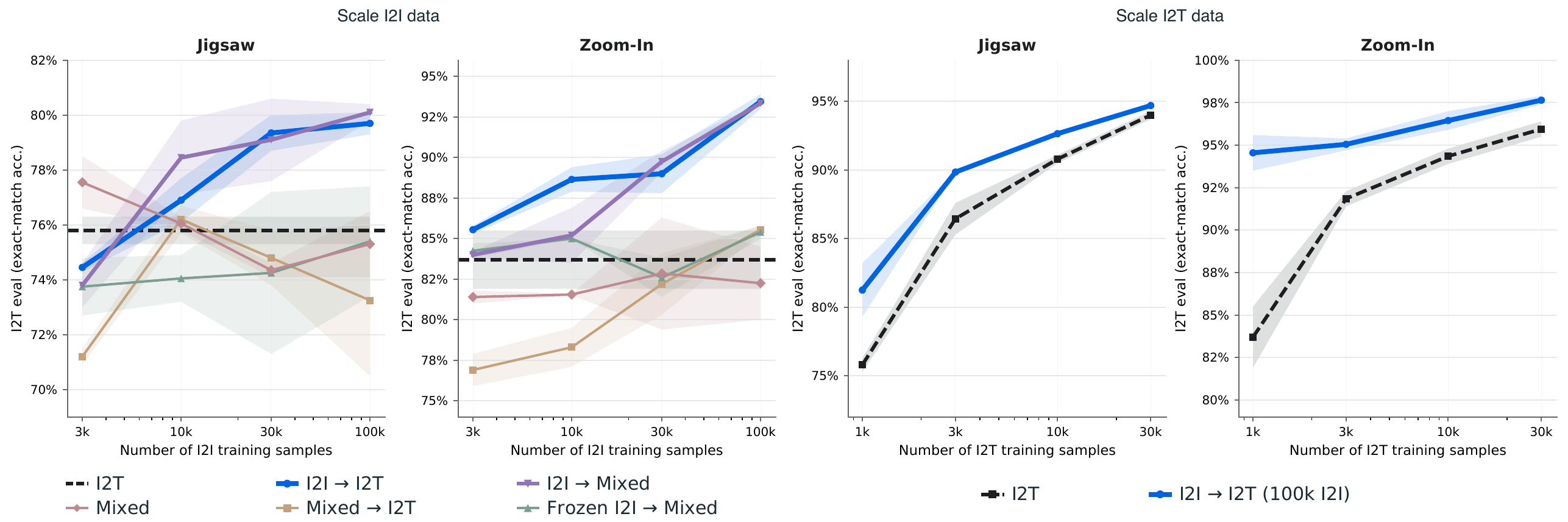
An initial I2I training stage that updates parameters shared with the I2T objective provides a useful initialization for subsequent I2T learning.

Finding 2

Visual generation supervision yields significant gains for specific visual understanding capabilities, through both related tasks and transfer across tasks.

Finding 3

Gradient alignment is concentrated in early pre-attention normalization layers and is positively associated with downstream transfer across both understanding capabilities and individual source-target pairs.
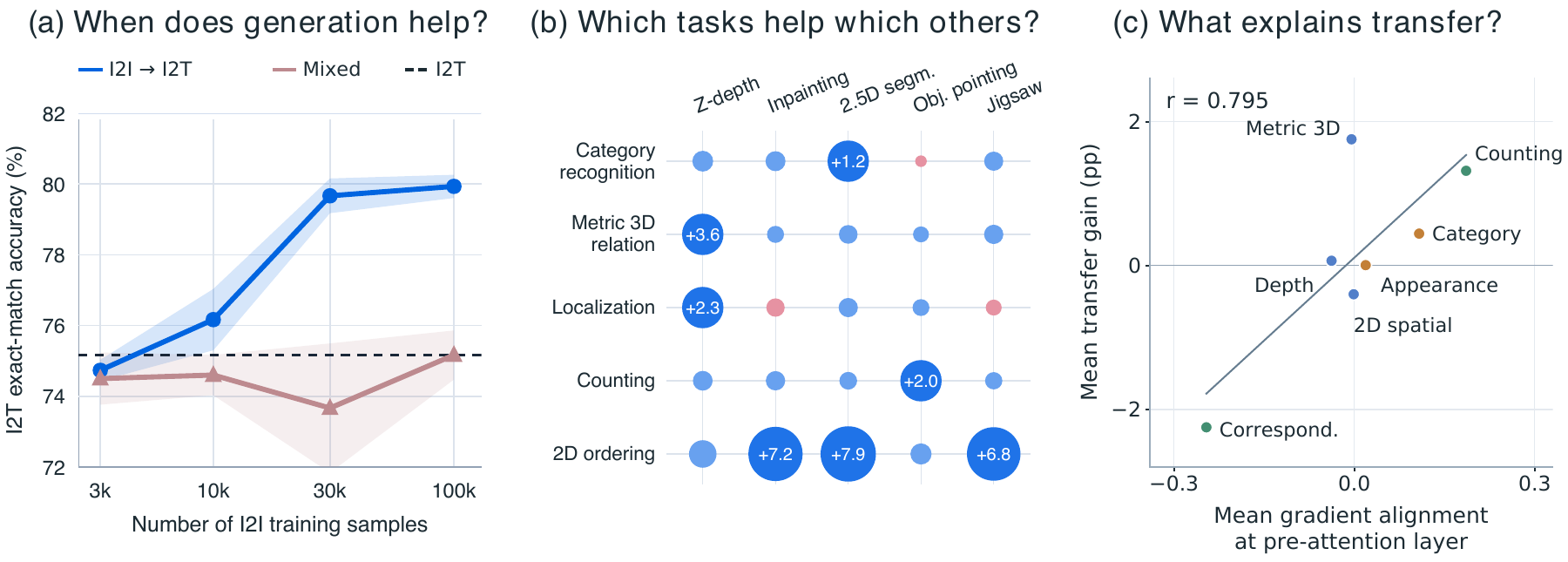
When and how does visual generation improve visual understanding?
blue: positivered: negative

Does visual generation help visual understanding?

To isolate the effect of confounding factors, we construct paired I2I and I2T tasks that require solving the same task from the same input, differing only in whether the answer is produced as an image or as text. This allows us to directly test whether supervision from an I2I objective transfers to the corresponding I2T task. This setup eliminates differences in annotation quality, image source, and other factors.

Controlled Jigsaw and Zoom-In tasks with image and text outputs.

In Jigsaw, patches of an image are shuffled, and the model must recover their spatial arrangement. In Zoom-In, views of the same image at different zoom levels are shuffled, and the model must recover their correct order.

For each input, the I2I objective produces the correctly ordered image, while the I2T objective predicts the same ordering as a permutation in text. The objectives require the same visual operation on the same input and differ only in output modality.
Which training recipe transfers best?

I2T accuracy versus I2I training examples across recipes, with 1k I2T examples. I2T accuracy versus I2T training examples for I2T-only and I2I → I2T training (100k I2I examples). Curves show means over three seeds. Shading indicates ±1 SEM.
I2T accuracy versus I2I training examples across recipes, with 1k I2T examples. I2T accuracy versus I2T training examples for I2T-only and I2I → I2T training (100k I2I examples). Curves show means over three seeds. Shading indicates ±1 SEM.1

We therefore use I2I → I2T as the default recipe in subsequent experiments.

An initial I2I training stage that updates parameters shared with the I2T objective provides a useful initialization for subsequent I2T learning.

OmniTaskonomy: A unified taxonomy of visual capabilities

Existing benchmarks typically organize visual tasks by task formulation or output modality, leaving visual generation and understanding tasks separated. This makes it difficult to compare and study tasks that rely on similar visual capabilities but produce different outputs. We introduce OmniTaskonomy, which organizes I2I tasks and understanding tasks in a shared hierarchy. For a visual understanding sample, we consider the primary visual capability required to solve it; for an I2I task, we consider the visual capability directly supervised by its training objective.

Click a node to explore
OmniTaskonomy
A unified taxonomy of visual tasks organized into three broad families: Recognition, Reconstruction, and Reorganization. I2I training objectives and understanding capabilities remain separate leaves, but share the same visual hierarchy.

Which generation tasks help which capabilities?

Hover to magnify · click to pinSwipe to explore · tap a cellNegativePositiveOutlined: p < 0.05 (two-sided paired permutation test vs. I2T-only)
I2I supervision task
RecognitionReconstructionReorganization
I2T capabilityObject editingAttribute editingColorizationZ-depthEuclidean depthSurface normalsPrincipal curvatureOcclusion edges3D keypointsReshadingInpaintingSemantic segmentation2D edges2D keypoints2D segmentation2.5D segmentationObject pointingJigsawLocalization
Category recognition
Appearance understanding
Visual similarity
State recognition
Activity understanding
Anomaly detection
Situation understanding
OCR and text recognition
Lighting understanding
Depth understanding
Metric 3D relation
Orientation understanding
2D spatial relation
Multi-view reasoning
Localization
Connectivity
Counting
2D Ordering
Visual correspondence

Visual generation supervision yields significant gains for specific visual understanding capabilities, through both related tasks and transfer across tasks.

Shared visual operations predict several of the strongest gains.

Localization and object pointing produce the largest improvements in counting (+2.5 and +2.0 pp), consistent with all three tasks requiring individual objects to be identified and spatially localized.

Similarly, Z-depth, Euclidean depth, and surface normals improve metric 3D relation by 3.6, 3.8, and 3.4 pp, respectively, connecting dense geometric reconstruction to relational 3D judgments. Jigsaw improves 2D ordering by 6.8 pp, consistent with both tasks requiring the relative spatial arrangement of image regions.

Useful transfer is not confined to closely matched capabilities.

Inpainting improves both counting (+1.5 pp) and 2D ordering (+7.2 pp), despite neither target explicitly requiring missing-region reconstruction. Solving inpainting tasks may encourage the model to infer object quantity and global spatial structure from incomplete local evidence. 2.5D segmentation likewise improves category recognition (+1.2 pp), potentially because capturing object boundaries can shape cues that support category recognition.

What explains visual generation-to-understanding transfer?

JigsawZoom-In
-0.10.00.20.40.6ViTConn. inConn. out2D pos.Pre-attnQKVQ normK normOutPre-MLPGateUpDown
Pre-attn RMSNormJigsaw 0.54Zoom-In 0.44
Gradient alignment for the controlled Jigsaw and Zoom-In pairs across model components and individual pre-attention RMSNorm layers.
Hover, tap, or focus a point to inspect itRecognitionReconstructionReorganization
Transfer by capabilityr = 0.795
-2-1012-0.3-0.1500.15Mean gradient alignment across 19 sourcesMean transfer gain (pp)Category recognition — alignment 0.108, transfer +0.44 ppCategory
Appearance understanding — alignment 0.019, transfer +0.01 ppAppearance
Depth understanding — alignment -0.038, transfer +0.07 ppDepth
Metric 3D relation — alignment -0.005, transfer +1.75 ppMetric 3D
2D spatial relation — alignment -0.001, transfer -0.40 pp2D spatial
Counting — alignment 0.186, transfer +1.32 ppCounting
Visual correspondence — alignment -0.246, transfer -2.25 ppCorrespondence

Mean gradient alignment versus mean transfer for seven understanding capabilities, averaging over 19 I2I sources.

Transfer by task pair133 pairs · r = 0.529
-6-303-0.5-0.2500.25Gradient alignmentTransfer gain (pp)Object editing → Category recognition — alignment 0.209, transfer +0.07 pp
Attribute editing → Category recognition — alignment 0.202, transfer +1.18 pp
Colorization (Taskonomy) → Category recognition — alignment 0.051, transfer +0.24 pp
Z-depth → Category recognition — alignment 0.125, transfer +1.04 pp
Euclidean depth → Category recognition — alignment 0.137, transfer +0.90 pp
Surface normals → Category recognition — alignment 0.011, transfer +0.14 pp
Principal curvature → Category recognition — alignment 0.105, transfer +0.03 pp
Occlusion edges → Category recognition — alignment 0.074, transfer -0.55 pp
3D keypoints → Category recognition — alignment 0.247, transfer +0.38 pp
Reshading → Category recognition — alignment 0.230, transfer +0.21 pp
Inpainting → Category recognition — alignment 0.142, transfer +0.94 pp
Semantic segmentation → Category recognition — alignment 0.247, transfer +0.66 pp
2D edges → Category recognition — alignment -0.205, transfer +0.69 pp
2D keypoints → Category recognition — alignment 0.042, transfer -0.10 pp
2D segmentation → Category recognition — alignment -0.002, transfer +0.38 pp
2.5D segmentation → Category recognition — alignment 0.084, transfer +1.25 pp
Object pointing → Category recognition — alignment 0.113, transfer -0.14 pp
Jigsaw → Category recognition — alignment 0.107, transfer +0.76 pp
Localization → Category recognition — alignment 0.131, transfer +0.35 pp
Object editing → Appearance understanding — alignment 0.053, transfer -0.82 pp
Attribute editing → Appearance understanding — alignment 0.064, transfer -0.53 pp
Colorization (Taskonomy) → Appearance understanding — alignment -0.038, transfer -0.24 pp
Z-depth → Appearance understanding — alignment -0.120, transfer -0.24 pp
Euclidean depth → Appearance understanding — alignment -0.120, transfer -0.15 pp
Surface normals → Appearance understanding — alignment 0.040, transfer +0.00 pp
Principal curvature → Appearance understanding — alignment 0.136, transfer +0.19 pp
Occlusion edges → Appearance understanding — alignment -0.009, transfer +0.29 pp
3D keypoints → Appearance understanding — alignment 0.222, transfer -0.73 pp
Reshading → Appearance understanding — alignment 0.115, transfer +0.10 pp
Inpainting → Appearance understanding — alignment 0.025, transfer +0.15 pp
Semantic segmentation → Appearance understanding — alignment 0.114, transfer +0.34 pp
2D edges → Appearance understanding — alignment -0.191, transfer +0.44 pp
2D keypoints → Appearance understanding — alignment 0.097, transfer -0.24 pp
2D segmentation → Appearance understanding — alignment -0.048, transfer -0.19 pp
2.5D segmentation → Appearance understanding — alignment 0.059, transfer +0.34 pp
Object pointing → Appearance understanding — alignment -0.025, transfer -0.29 pp
Jigsaw → Appearance understanding — alignment -0.023, transfer +1.50 pp
Localization → Appearance understanding — alignment 0.008, transfer +0.19 pp
Object editing → Depth understanding — alignment 0.014, transfer -0.04 pp
Attribute editing → Depth understanding — alignment -0.005, transfer -0.61 pp
Colorization (Taskonomy) → Depth understanding — alignment -0.073, transfer +0.00 pp
Z-depth → Depth understanding — alignment 0.070, transfer +0.00 pp
Euclidean depth → Depth understanding — alignment 0.147, transfer +0.81 pp
Surface normals → Depth understanding — alignment -0.135, transfer -0.24 pp
Principal curvature → Depth understanding — alignment -0.114, transfer +0.93 pp
Occlusion edges → Depth understanding — alignment -0.095, transfer +0.65 pp
3D keypoints → Depth understanding — alignment -0.080, transfer +0.49 pp
Reshading → Depth understanding — alignment 0.032, transfer -0.12 pp
Inpainting → Depth understanding — alignment -0.065, transfer -0.85 pp
Semantic segmentation → Depth understanding — alignment 0.093, transfer -1.18 pp
2D edges → Depth understanding — alignment -0.076, transfer +0.73 pp
2D keypoints → Depth understanding — alignment -0.067, transfer +0.89 pp
2D segmentation → Depth understanding — alignment -0.126, transfer +0.77 pp
2.5D segmentation → Depth understanding — alignment -0.103, transfer -0.28 pp
Object pointing → Depth understanding — alignment -0.038, transfer -1.99 pp
Jigsaw → Depth understanding — alignment -0.061, transfer +0.41 pp
Localization → Depth understanding — alignment -0.040, transfer +0.89 pp
Object editing → Metric 3D relation — alignment -0.059, transfer +2.03 pp
Attribute editing → Metric 3D relation — alignment -0.086, transfer +0.60 pp
Colorization (Taskonomy) → Metric 3D relation — alignment -0.283, transfer +0.46 pp
Z-depth → Metric 3D relation — alignment 0.045, transfer +3.60 pp
Euclidean depth → Metric 3D relation — alignment 0.169, transfer +3.83 pp
Surface normals → Metric 3D relation — alignment -0.040, transfer +3.41 pp
Principal curvature → Metric 3D relation — alignment -0.002, transfer +1.34 pp
Occlusion edges → Metric 3D relation — alignment -0.096, transfer +1.84 pp
3D keypoints → Metric 3D relation — alignment -0.061, transfer +1.38 pp
Reshading → Metric 3D relation — alignment 0.094, transfer +1.75 pp
Inpainting → Metric 3D relation — alignment -0.072, transfer +1.01 pp
Semantic segmentation → Metric 3D relation — alignment 0.070, transfer +1.94 pp
2D edges → Metric 3D relation — alignment 0.080, transfer +1.20 pp
2D keypoints → Metric 3D relation — alignment 0.137, transfer +0.97 pp
2D segmentation → Metric 3D relation — alignment 0.032, transfer +1.06 pp
2.5D segmentation → Metric 3D relation — alignment 0.044, transfer +2.17 pp
Object pointing → Metric 3D relation — alignment -0.021, transfer +0.32 pp
Jigsaw → Metric 3D relation — alignment -0.019, transfer +2.63 pp
Localization → Metric 3D relation — alignment -0.019, transfer +1.80 pp
Object editing → 2D spatial relation — alignment 0.037, transfer -1.62 pp
Attribute editing → 2D spatial relation — alignment 0.045, transfer -0.58 pp
Colorization (Taskonomy) → 2D spatial relation — alignment -0.176, transfer -1.22 pp
Z-depth → 2D spatial relation — alignment -0.137, transfer -0.79 pp
Euclidean depth → 2D spatial relation — alignment -0.102, transfer -0.58 pp
Surface normals → 2D spatial relation — alignment 0.008, transfer -0.58 pp
Principal curvature → 2D spatial relation — alignment 0.079, transfer +0.40 pp
Occlusion edges → 2D spatial relation — alignment -0.078, transfer -1.11 pp
3D keypoints → 2D spatial relation — alignment 0.164, transfer +0.07 pp
Reshading → 2D spatial relation — alignment 0.068, transfer +0.00 pp
Inpainting → 2D spatial relation — alignment 0.035, transfer -0.40 pp
Semantic segmentation → 2D spatial relation — alignment 0.108, transfer -0.32 pp
2D edges → 2D spatial relation — alignment -0.170, transfer +0.50 pp
2D keypoints → 2D spatial relation — alignment 0.140, transfer +0.32 pp
2D segmentation → 2D spatial relation — alignment -0.060, transfer -0.07 pp
2.5D segmentation → 2D spatial relation — alignment 0.006, transfer -0.68 pp
Object pointing → 2D spatial relation — alignment -0.008, transfer -0.14 pp
Jigsaw → 2D spatial relation — alignment -0.005, transfer -0.22 pp
Localization → 2D spatial relation — alignment 0.024, transfer -0.58 pp
Object editing → Counting — alignment 0.282, transfer +1.08 pp
Attribute editing → Counting — alignment 0.270, transfer +1.45 pp
Colorization (Taskonomy) → Counting — alignment 0.085, transfer +0.73 pp
Z-depth → Counting — alignment 0.259, transfer +1.58 pp
Euclidean depth → Counting — alignment 0.245, transfer +0.97 pp
Surface normals → Counting — alignment 0.086, transfer +1.28 pp
Principal curvature → Counting — alignment 0.195, transfer +0.82 pp
Occlusion edges → Counting — alignment 0.140, transfer +1.02 pp
3D keypoints → Counting — alignment 0.311, transfer +1.49 pp
Reshading → Counting — alignment 0.303, transfer +1.19 pp
Inpainting → Counting — alignment 0.200, transfer +1.49 pp
Semantic segmentation → Counting — alignment 0.317, transfer +1.08 pp
2D edges → Counting — alignment -0.161, transfer +1.53 pp
2D keypoints → Counting — alignment 0.074, transfer +1.41 pp
2D segmentation → Counting — alignment 0.160, transfer +1.43 pp
2.5D segmentation → Counting — alignment 0.206, transfer +1.06 pp
Object pointing → Counting — alignment 0.191, transfer +1.97 pp
Jigsaw → Counting — alignment 0.173, transfer +0.95 pp
Localization → Counting — alignment 0.198, transfer +2.49 pp
Object editing → Visual correspondence — alignment -0.319, transfer -2.03 pp
Attribute editing → Visual correspondence — alignment -0.287, transfer -2.30 pp
Colorization (Taskonomy) → Visual correspondence — alignment -0.052, transfer -0.92 pp
Z-depth → Visual correspondence — alignment -0.520, transfer -1.38 pp
Euclidean depth → Visual correspondence — alignment -0.501, transfer -4.59 pp
Surface normals → Visual correspondence — alignment -0.026, transfer -2.89 pp
Principal curvature → Visual correspondence — alignment 0.039, transfer -1.31 pp
Occlusion edges → Visual correspondence — alignment -0.173, transfer -0.59 pp
3D keypoints → Visual correspondence — alignment -0.207, transfer -4.33 pp
Reshading → Visual correspondence — alignment -0.289, transfer -3.02 pp
Inpainting → Visual correspondence — alignment -0.273, transfer -1.84 pp
Semantic segmentation → Visual correspondence — alignment -0.186, transfer -4.00 pp
2D edges → Visual correspondence — alignment -0.244, transfer -2.62 pp
2D keypoints → Visual correspondence — alignment -0.155, transfer -0.26 pp
2D segmentation → Visual correspondence — alignment -0.273, transfer -3.61 pp
2.5D segmentation → Visual correspondence — alignment -0.256, transfer -5.51 pp
Object pointing → Visual correspondence — alignment -0.333, transfer +1.71 pp
Jigsaw → Visual correspondence — alignment -0.318, transfer -2.89 pp
Localization → Visual correspondence — alignment -0.301, transfer -0.33 pp
2D edges → Category recognitionObject pointing → Counting3D keypoints → Appearance2.5D segmentation → Correspondence

Alignment and transfer for all 133 source–target pairs.

average alignment and average transfer are strongly positively correlated across the seven capabilities (r=0.795). Capabilities whose gradients are more compatible with generation objectives, on average, therefore, also tend to receive larger gains from I2I training.

Alignment and transfer are positively correlated across these 133 pairs (r=0.529).

Gradient alignment is concentrated in early pre-attention normalization layers and is positively associated with downstream transfer across both understanding capabilities and individual source-target pairs.

Citation

% BibTeX pending.